What Is a Bonding Curve in Crypto and How Does It Work?

Programs and platforms built on blockchains are continuously looking for ways to become more decentralized and automated. Currently, many protocol ecosystems still require external entities such as exchanges to carry out some of their functions. By employing smart contracts, blockchains have been able to move many functions into a more automated and decentralized sphere. Moreover, increased use of mathematical algorithms is allowing for a broader range of transactions to be carried out without any human or external interference. This progress is allowing for blockchain protocol ecosystems to become increasingly independent, decentralized, and automated. One mathematical concept that is starting to make waves in this space is an automated market maker (AMM) known as a bonding curve.

What Is a Bonding Curve?

Initially conceived by Simon de la Rouviere in 2017, a bonding curve is a mathematical concept that can be inbuilt into platforms and applications to calculate a token’s value as determined by its supply. Investors will buy tokens, according to the price listed on the bonding curve, in exchange for collateral in fiat currencies of other cryptos, such as Bitcoin (BTC) and Ethereum (ETH). The bonding curve’s value estimate of the token is taken when investors buy tokens (where they are minted) and when they sell tokens (where they are burned). As these bonding curve tokens are minted and burned, the supply changes, which will in turn be reflected in the value listed by the bonding curve.

Bonding curves have multiple functions:

• Improving valuations:Bonding curves are transparent as they are inbuilt into blockchains, and they are predictable and accurate as they are built using math. Bonding curves are also a dynamic approach to calculating cryptocurrency values, as they take ecosystem growth into consideration. A bonding curve recognizes that as an ecosystem grows, so does the amount of that ecosystem’s token, and subsequently so does its value.

• Pre-setting how token value will increase or decrease:A bonding curve states that token and coin prices will change with their supply, either decreasing or increasing, thereby creating a continuous token model. If a developer wants to take more control over this aspect, they can choose a specific bonding curve shape, which will determine how much a token’s value will increase based on supply.

• Removing the need for exchanges:As a fully automated market maker (AMM), bonding curves not only allow for the calculation of a token’s price, but also enable transactions. The mathematical algorithm estimates the cost of the token, which it shows to the investor. After this, the investor can simply buy or sell their tokens right there. This function is very exciting, as it moves cryptocurrency further away from centralization.

• Allowing for multiple tokens in one ecosystem: Another function of a bonding curve is that by minting its own tokens, it can allow for multiple tokens to be used within one ecosystem. A developer can build multiple bonding curves into the ecosystem, thereby allowing for different tokens to be used for different projects, according to the functionality that the developer wants. This allows for greater versatility as different tokens can be used across different blockchains, depending on the usage of the token and the smart contracts or two-way pegs that connect the blockchains.

How Does a Bonding Curve Work?

A simple linear bonding curve states that x = y, which is to say, token supply = token value. This means that token number 10 will cost $10 and token number 20 will cost $20. However, this does not mean that if an individual buys 10 tokens, they will pay $10. Token 1 will cost $1, token 2 will cost $2, token 3 will cost $3, and so on. Thus, if an individual wants to buy 10 tokens, they will have to pay the price of each of those 10 tokens, which would be $1+$2+$3+$4+$5…, totalling a cost of $55. If an individual wants to buy 10 coins, but 10 have already been purchased, then the individual in question would buy from token 11 to token 20. This means that they would pay $11+$12+$13+$14…, totalling $155. Thus, this type of linear bonding curve gives higher profit to early investors.

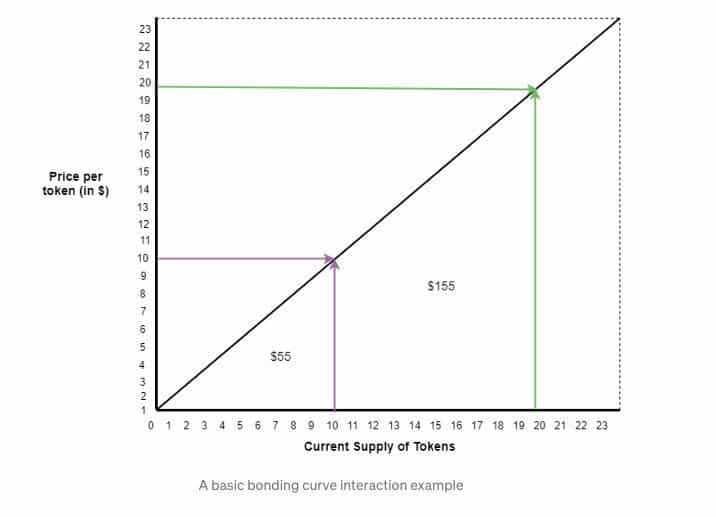
A linear bonding curve

If these investors were to sell, the early investor would make a larger profit.

The early investor bought 10 tokens for $55, but with the subsequent investment from the second individual, the token value went up. This means that the first investor can sell at the new, higher value.

Once the first investor sells their tokens, these are burnt, which means that there are less tokens in circulation. The supply has therefore decreased, meaning that the value has too. The second investor who bought their 10 tokens for $155 would therefore lose money if they sold at this point.

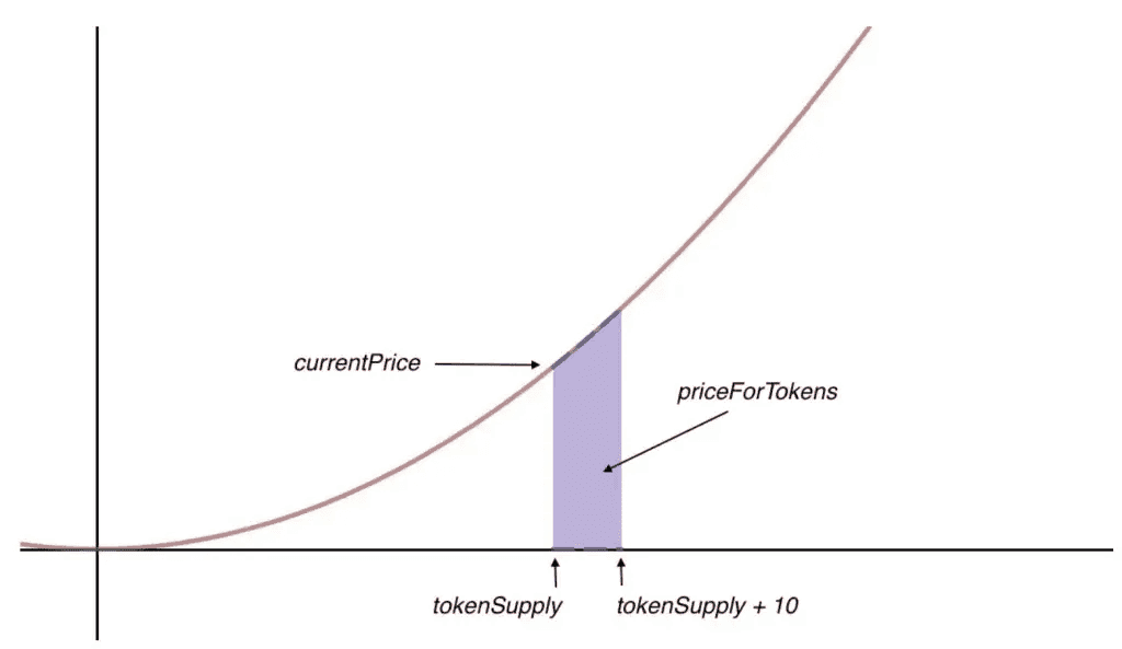
A bonding curve allows for investors to buy or sell their tokens at any point in time, but as with any investment, this could result in profit or loss depending on the market. When building their programs, developers can control how much profit or loss an investor will make depending at which point in the bonding curve they make their transaction. This is done by choosing a particular shape for the bonding curve.

Applications of Bonding Curves in Crypto

Bonding curves first gained attention around 2017–2018 when projects looked for new ways to raise funds and bootstrap markets. Since then, they’ve been applied in various contexts:

Token Sales and Initial Offerings: A bonding curve allows continuous token sales, differentiating from traditional ICOs where a fixed number of tokens are sold at a set price. Early supporters can buy tokens at lower prices, with prices rising as demand increases, linking funding directly to interest. For instance, Fairmint’s Continuous Organization lets companies raise funds through a bonding curve. Another example is Pump.fun, which creates a bonding curve for meme coins on Solana, ensuring liquidity and smooth price increases without needing exchange listings.

Automated Market Makers (DEXes): Platforms like Uniswap and Curve Finance implement bonding curve principles for trading pairs. Uniswap’s constant product formula functions as a bonding curve, while Curve optimizes for stablecoin trading with a flat curve to minimize slippage. These DEXs showcase the success of bonding curve mechanisms in offering deep liquidity and enabling substantial trading volumes without intermediaries.

Bonding Curve in Tokenomics (source)

Stablecoins (Algorithmic): Some algorithmic stablecoins, like the failed TerraUSD, employed bonding curve logic to maintain pegs by adjusting supply based on demand. However, this can lead to risks, as seen in UST’s catastrophic loss of its peg. Other projects, such as Ampleforth, use similar supply adjustments to target price maintenance.

Governance and DAO Tokens: Bonding curves can also fund DAOs. Individuals pay into the curve for governance tokens, with prices rising as more participants join. This creates an evolving membership model, where exiting members can sell back to the curve. Projects like DAOstack and CommonStack have utilized this method to manage member dynamics while maintaining value for remaining participants.

NFTs and Digital Art: In the NFT space, bonding curves have been used to gradually increase prices as more editions are sold. This model incentivizes early collectors with lower prices but has faced criticism in some applications.

What are the Types of Bonding Curves?

A linear bonding curve is perhaps the simplest, but depending on what the developer wants to accomplish, they might want to encourage early investment or discourage early selling, among other things. As a bonding curve is inbuilt into the blockchain and is unchangeable, the shape it takes will determine these aspects when investors buy and sell.

There are four most used bonging curves:

1. Sigmoid curve

2. Quadratic curve

3. Negative exponential curve

4. Linear (non-increasing) curve

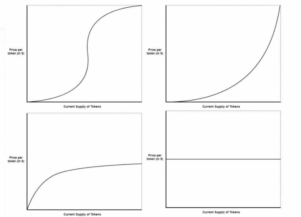
Four of the most popular bonding curves: Sigmoid (top left); quadratic curve (top right); negative exponential curve (bottom left); and linear (non-increasing) curve (bottom right). (Source: medium.com)

Different bonding curve shapes will be adopted based on what type of investment the developer is looking for (see above image for graphics of the below discussed bonding curves):

• To reward early investors:If a developer wants to reward early investors, they can use a sigmoid or quadratic bonding curve. These bonding curves are particularly good for projects that a developer expects to go viral. These could be projects that are geared toward quite a large audience, for example a platform that revolves around gaming in crypto like GameFi, a platform that creates and sells non-fungible tokens (NFTs) like ECOMI, or an audio sharing platform like Audius. Here, a developer could use a sigmoid curve to keep costs low for early investors, while dramatically increasing the cost once reaching the more mainstream adopters. This can be seen by the sharp increase in price at the inflection point in the sigmoid curve. Alternatively, they could use a quadratic bonding curve to offer a steadier increase that is still significantly lower for early investors than latecomers.

• To incentivize early investment but not disincentivize later investment:If a developer is using a bonding curve for a project that requires a long period of investment, for example a fundraising project, then they might use a negative exponential curve or a linear bonding curve. By using a negative exponential curve, the developer incentivizes the investor by giving them a chance to buy-in at a low cost and make a profit on their investment. As the project gathers more interest and more investment, the curve begins to flatten, finally only having a gradual increase. With a linear bonding curve, the developers will have a steady increase in cost as the project gathers more investors. A linear bonding curve is also more profitable for early investors, but there is not such a large contrast between costs for early and late investors as with the sigmoid and quadratic curves.

• To keep costs continuous:A linear (non-increasing) bonding curve can be used for projects where investors are not looking to make or lose money from that investment. Here, the cost remains steady meaning no loss or profit is made. This type of bonding curve could work well for investors who are simply supporting a project that they believe in.

Advantages of Bonding Curves

1. Continuous Liquidity: Bonding curves provide a guaranteed price for buying or selling tokens directly from the contract, ensuring liquidity without the need for market makers or exchanges.

2. Fair and Transparent Pricing: The pricing formula is public and predefined, ensuring fairness as everyone faces the same conditions. This transparency builds trust, as the logic is immutable on-chain.

3. Bootstrap Funding: Bonding curves enable projects to fundraise effortlessly, automatically managing token sales and allowing funding to align with actual interest over time.

4. Incentivize Early Adoption: Early adopters benefit from lower prices in a structured way, fostering a supportive community invested in the project’s success.

5. Automatic Market Making: In DeFi, bonding curves facilitate automated exchanges, democratizing liquidity provision and reducing reliance on traditional market-making infrastructure.

6. Predictability for Token Economics: Projects can simulate demand scenarios to estimate pricing and funding, providing a stable tokenomics framework that can reduce speculative volatility.

7. Aligning Value with Usage: Bonding curves can link token value to system participation, creating a cycle where increased participation raises token prices, rewarding users.

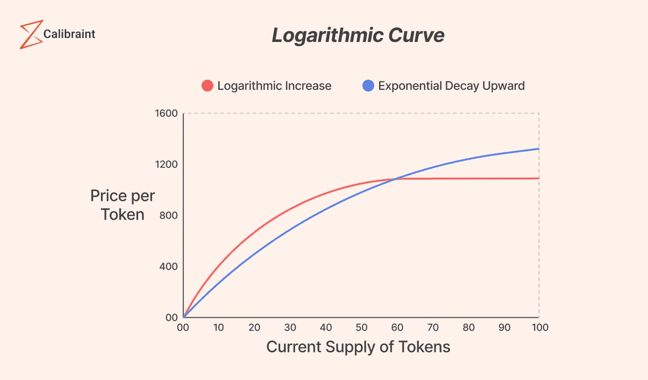
Logarithmic Bonding Curve (source)

Risks and Challenges of Bonding Curves

While bonding curves are powerful, they are not magic and they come with their own set of risks and considerations:

1. Volatility and Speculation: Exponential bonding curves can lead to extreme price fluctuations, encouraging speculation. Early holders might sell off tokens to realize profits, causing prices to drop and harming latecomers who bought high.

2. Whale Manipulation: Large buyers or sellers can significantly impact prices on bonding curves. A whale buying a large number of tokens can inflate prices for later buyers, while selling off can crash the price, making such curves sensitive to large transactions.

3. Liquidity vs. Price Impact: While bonding curves generally offer good liquidity, larger trades can cause considerable price slippage, especially on steep curves or with smaller reserves.

4. Smart Contract Risk: Bonding curves rely on complex smart contracts, which may contain vulnerabilities. A bug could allow token minting without proper exchange or compromise reserve assets, creating a risk for users.

5. Capital Inefficiency: Some models lock funds as reserves for liquidity, leading to opportunity costs. Mismanagement can cause reserves to inadequately cover token supply, impacting confidence.

6. Complexity and User Understanding: Bonding curves can confuse users, particularly those unfamiliar with the concepts. Users may overpay or panic sell if they don't understand how their actions affect prices.

7. Potential for Bank Run Dynamics: In cases of reduced confidence, especially in stablecoin systems, a sudden rush to sell can lead to a price crash if reserves are low.

8. Regulatory Considerations: Bonding curves could be seen as securities offerings, attracting regulatory scrutiny, particularly if bought with profit expectations. Compliance is essential.

9. Arbitrage and External Market Effects: If tokens trade on other platforms, price discrepancies could arise, leading to arbitrage opportunities.

Conclusion

Bonding curves are a type of AMM. They use automated algorithmic trading to calculate the value of a token according to the pre-established bonding curve shape and the token supply. This means that an investor can buy tokens using collateral, and then sell their tokens whenever they want, all directly through the program. This reduces any human error, as it’s automated and uses math, creates a completely transparent trading process, and keeps it decentralized since it’s all carried out through smart contracts. Bonding curves are a way for developers to implement their own investment strategies in a transparent and error-free way, without the need for an exchange. In addition, bonding curves can help investors predict how much their assets could rise in value, and thus calculate their potential profits. It is important to note, however, that although a bonding curve can show how much an asset could rise, it cannot guarantee that the coins will be bought, and thus it does not guarantee that it will hit that value.

In summary, bonding curves have proven to be a powerful concept for aligning incentives and enabling fluid markets in the crypto space. They embody the spirit of DeFi: removing middlemen and encoding financial logic directly on blockchain. For users, the key takeaway is that bonding curves are all about the interplay of supply and demand coded into an algorithm. If you participate in a token sale or DeFi protocol using bonding curves, understanding the specific curve and its implications will help you make informed decisions.